These are important questions I'm sure you ask yourself or you frequently hear from your stakeholders.
A/B testing is a time-consuming and expensive process. Don’t get me wrong, it is well worth the effort. But let’s be honest, by the time you’ve reached the point of working out how long you should run a test, you will have already spent hours researching customer pain points, choosing a testing tool and building and designing your test variants. Therefore, it’s crucial not to let your hard work and investment go to waste by calling your tests too early.
It may sound surprising but it’s not uncommon for businesses to conclude a test too early, implement what they think is a winning test variation, only for the uplift to be eroded weeks later. The example below helps to illustrate this:

In the first two weeks of the test, the variation immediately outperforms control - maybe even gives you a statistically significant reading - and excitement builds for a new design that will boost conversions by 10%. However, leave it a little longer and notice how after 3-4 weeks the results start to converge with no significant improvement in our variation. Scenarios like this are not only frustrating but also expensive, with poor methodologies such as these costing retailers $13bn a year, as outlined by Qubit.
As a rule of thumb, you do not want to be running tests for under 4 weeks or over 6 weeks. Under 4 weeks isn’t long enough to account for variability and business cycles, and over 6 weeks risks cookie expiry leading to users possibly entering multiple variations jeopardising the results.
However, this is just a guide, there are actually four interlocking variables you really need to understand and consider in order to run a statistically viable A/B test.
- Baseline conversion rate
- Statistical significance level
- Statistical power
- Minimal detectable effect
I’ll now explain how these variables should be approached and calculated before you even think about launching a test.
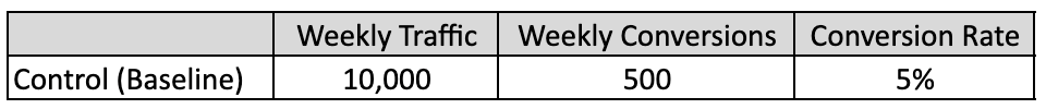
This is simply the traffic volume and conversion rate on the control - your current live website. When calculating time to run, this data will act as your baseline.
Statistical significance represents the likelihood that the difference in conversion rates between a given variation and the baseline is not due to chance. Industry norms are to aim for 95% statistical significance to be confident in implementing the correct winner.
For example, 95% statistical significance means we can be 95% confident that the results we see are due to an actual change in behaviour, not just random chance.
Although, it’s important to remember that just because a test has reached 95% statistical significance, it does not mean we automatically have a valid result.
In any given experiment there are actually 3 possible outcomes
- Accurate results - results are valid and we can stop test.
- False positive - results show a statistically significant effect, which doesn’t actually exist.
- False negative - results show no statistically significant change, when in fact there is one.
Too often testers stop as soon as their calculators tell them the golden 95% statistical significance has been reached - the prime reason for invalid test results. Yes, statistical significance is one checkpoint that must be met for valid results but, as we demonstrate below, it must be viewed in context with your baseline site performance, statistical power and minimal detectable effect before any test can be called.
Statistical power is defined as the probability of observing a statistically significant result, if a true effect of a certain magnitude is present. More simply, it’s the ability to detect a difference between test variations when a difference actually exists, and it is vital to pre-test planning.
Before we can really understand how we can use statistical power, we first need to know what we mean by a false positive or negative. Below are explanations of each:
- A false positive rejects the null hypothesis (the hypothesis that there is no significant difference between variations) when in fact it is actually true.
- In other words, our test is detecting a difference between variations but, in reality, it doesn't exist.
- False positives are linked with the statistical significance level. For example, for a test with a 95% confidence level, we only have a 5% probability of a false positive.
- A false negative is a failure to reject a null hypothesis that is actually false.
- In other words, our test does not find a significant improvement in the variation, however an improvement does actually exist.
So what does statistical power mean for your testing? It means you need to be aware of the balancing act between statistical significance and statistical power. The two have an inverse relationship with false positives (type 1 error) and false negatives (type 2 error).
Say, for example, that you wanted to increase the statistical significance from 95% to 99% on one of your tests, to really minimise your chances of getting a false positive. That would be perfectly reasonable but you would consequently increase your chances of getting a false negative. In other words, your test would be ‘underpowered’ and you might not reject the null hypothesis even though it is false!
You could further increase your statistical power to get around this, but each increase in power requires a corresponding increase in the sample size and the amount of time the test needs to run, and it’s likely these won’t be available.
So, as a general guideline, the industry standard is to set statistical power at 80%. With 80% power, we have a 20% probability of not being able to detect an uplift if there is one to be detected. However, as we’ll see in an example further down, you can use the A/B test calculator to adjust the other 3 elements - baseline figures, statistical significance and minimal detectable effect - to ensure you’ll get viable results while keeping with 80% power.
The MDE is the amount of effect the variation will need to deliver in order to achieve statistical significance given the power and sample size.
For example, if your baseline conversion rate is 10% and we estimate that our new variation will improve the baseline by at least 5%, our MDE is 5%.
The challenge is that the smaller the MDE the more difficult it is to detect a change, therefore requiring a larger sample size to retain the same power and statistical significance (i.e. validity of test). That means MDE has a real impact on the amount of traffic required to reach statistical significance.
Let’s look at an example - imagine you wanted to test a colour change of one word on a page. That’s a tiny change that will have minimal impact on your conversion rates, so it will therefore need a large sample in order to be detected. On the other hand, if you did a complete page redesign - an obvious change delivering a big effect - you’d only need a small sample size to detect the changes to your conversion rates and give you a statistically valid result.
Now we have an understanding of the key elements used to calculate our test run time, let’s look at how we actually calculate it.
First step is to find an A/B test calculator - I recommend CXL’s.
Using dummy figures, here are our parameters:
- Baseline conversion rate: 5%
- Statistical significance level: 95%
- Statistical power: 80%
- MDE: dependent on the above 3 parameters
Using an A/B test calculator, we can now use this data to give us our MDE which will tell us on how long our test should run and what degree of changes need to be present on the page, given the traffic volume and number of variations.
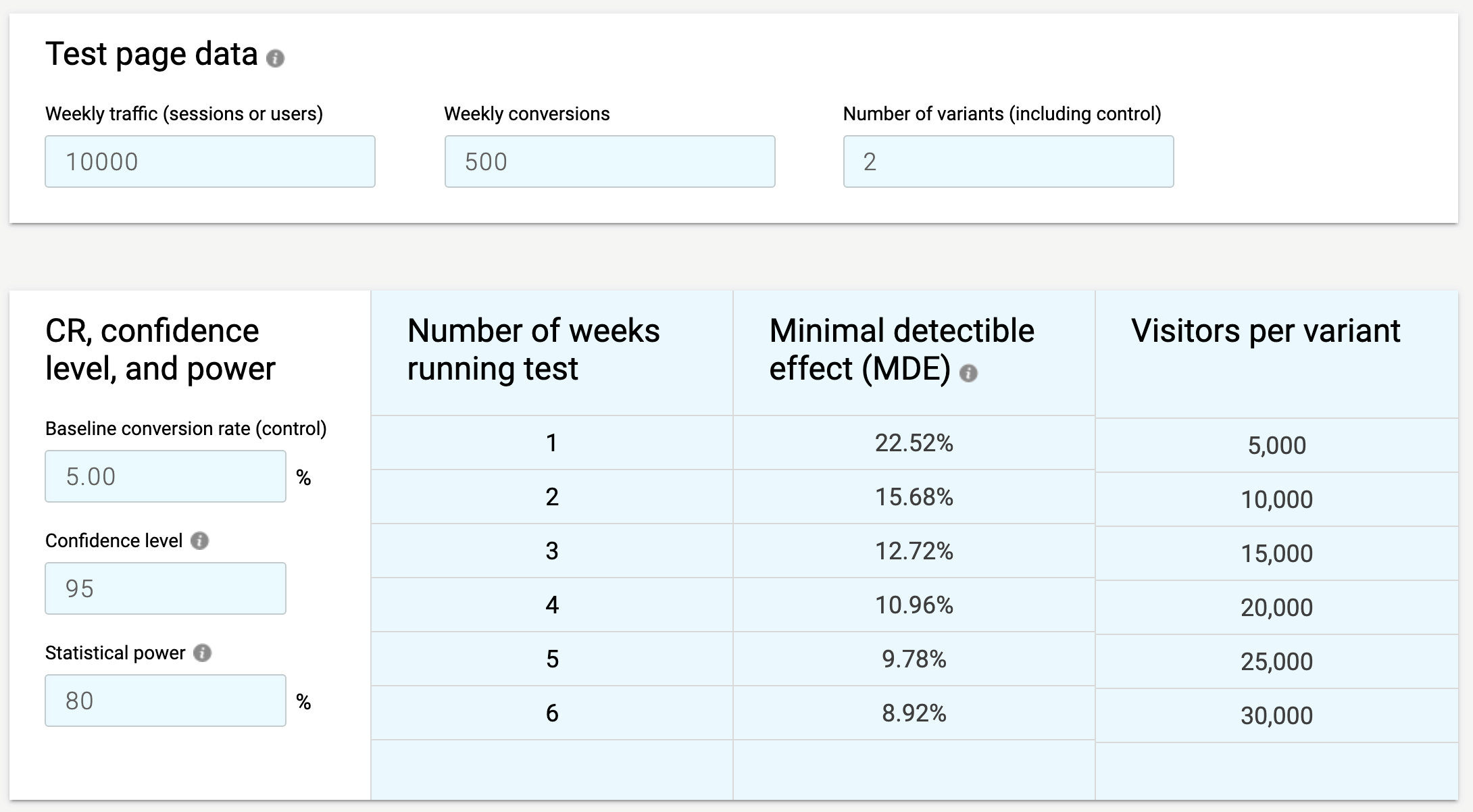
The tables below are straight from the A/B test calculator and show us that with a weekly traffic figure of 10,000 we would need to meet the following MDEs at 4 weeks in our test variations in order to get a 95% statistically significant result at 80% power.
Control + 1 Variation:
Control + 2 Variations:

Control + 3 Variations:
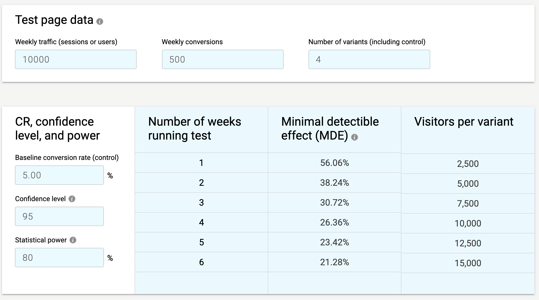
To put it more simply, if we run 3 variations we would need a larger MDE and therefore a much higher contrast test in order to reach accurate results after 4 weeks compared to if we ran 1 variation.
Far too often optimisers stop tests as soon as they hit 95% statistical significance. While this may seem like a rigorous process, it actually leaves your tests open to false positives and negatives. What this article explains is that running a statistically viable testing programme requires a few more considerations, plus an A/B test calculator. Taking the time to understand how to balance all these elements in your pre-test analysis will save time and money. And your users will thank you for it.
Optimisation Manager, Daydot